SAP Data replication in GCP using SLT and Data Intelligence

As organizations increasingly rely on cloud-based analytics, integrating enterprise data from SAP ERP systems like SAP ECC and SAP S/4HANA into cloud platforms like Google Cloud Platform (GCP) is crucial. This integration enables advanced analytics, real-time insights, and improved decision-making. There are several methods to achieve this data ingestion, some of them are opensource or cloud based solution — such as Airbyte , Google Data Fusion, Azure Datafactory, Amazon AppFlow - but we generally face challenges with continuous compatibility due to SAP’s frequent updates.
In fact, SAP is continuously updating its technologies, which can lead to open-source or third-party cloud solutions failing to work seamlessly with new SAP releases. This necessitates robust, adaptable solutions that can keep pace with SAP’s evolving ecosystem. For instance, the Data Fusion connector or Airbyte often struggles with Delta mode, creating reliability issues
This article explores one approach to achieving near real-time replication of SAP data to BigQuery using SAP-native solutions: SAP Landscape Transformation Replication Server (SLT) and SAP Data Intelligence (DI), though SAP Data Services can also be used as an alternative.
We will explain the significance of SAP data, followed by a step-by-step guide on setting up the SLT server and preparing a pipeline in Data Intelligence to extract and make the data available for business purposes.
Let’s start 🚀 !
1. Why SAP data is important :
The abbreviation SAP stands for Systems, Applications, and Products in Data Processing. SAP is a market leader in ERP software and is used by 93% of the Forbes Global 2000 companies. It is used by organizations big and small who are focused on improving operational efficiency and improving their bottom line, in a variety of verticals including manufacturing, retail, healthcare, finance, and more.
A great advantage of SAP software is that it has a lot of integrated ERP modules, each dealing with a particular aspect of business:
- Financial Accounting (FI): Managing financial transactions, financial reporting, and analysis.
- Controlling (CO): Management accounting and reporting, profitability analysis.
- Sales and Distribution (SD): Managing sales processes like order processing, pricing, and billing.
- Material Management (MM): Managing procurement processes- purchasing, inventory etc.
- Production Planning (PP): Managing production processes — scheduling products, material requirements
- Quality Management (QM): Managing quality control processes, quality control and inspection
- Plant Maintenance (PM): Managing plant maintenance processes, preventive maintenance etc.
- Human Capital Management (HCM): Managing human resource processes, managing talent, payroll etc.
- Project System (PS): Managing project planning, execution, and monitoring, allocating resources
- Business Warehouse (BW): Data warehousing and business intelligence capabilities
Apart from these SAP ERP modules, there could be other add-on modules for specific industries and business operations. As you can see, having an SAP implementation can be instrumental in providing a holistic 360-degree view of data. Every department has access to a unified accurate view of data and can query the data leading to actionable, effective insights.
In my career, I have worked for five companies, and four of them used SAP systems (SAP Concur, SAP ECC, and SAP S/4HANA) and it’s was important to implement solutions to extract SAP data for their analytics workload
2. Architecture High Level Overview:
As explained in the introduction, in order to develop an end-to-end pipeline to replicate SAP data , we use two SAP native solutions in order to export data from SAP to GCP and then a simple batch load in GCP side to ingest data into Bigquery. The solution works for batch or near realtime ingestion.
The proposed solution is explained in the following diagram:

We start by deploying SLT in a dedicated server, which will configure triggers on the relevant SAP object and changes to the object in SAP will then be captured and stored in the queue in the SLT server for an ODP (Operational Data Provisioning) scenario. SAP DI will poll this queue on a preconfigured schedule to synchronize these changes to a Cloud Storage objects. At the end, there is a batch job that push storage files to Biquery.
⚠️ As shown in the diagram (on the left side), we distinguish between two types of objects in SAP: tables and CDS (Core Data Services) Views.
- Tables: These are database objects that store transactional or master data in rows and columns, much like traditional relational database tables or BigQuery tables. For example, tables like MARA (Material Master) or EKPO (Purchase Order Items) store business data directly in the database.
- CDS Views: Unlike tables, CDS views do not store data. Instead, they are virtual data models (views) that define how data is retrieved from one or more SAP tables or other sources. The data is fetched from the underlying tables at runtime when the CDS view is executed. CDS views are defined using SQL-like syntax, similar to BigQuery views.
The extraction process differs for views and tables. While most of this article focuses on replicating SAP tables, we will explain briefly in the final section how to retrieve data from CDS Views.
Now, let’s dive into the details of each component of our architecture!
2.1 SAP SLT
SAP SLT refers to the SAP Landscape Transformation Replication Server, a component of the SAP Business Technology Platform that simplifies the entire data replication process and facilitates better connections between SAP system and non-SAP system operations. The LT Replication Server is an Extract, Transform, Load (ETL) tool that delivers real-time data using trigger-based Change Data Capture (CDC) functionality and allows users to load and replicate data from an SAP source system or non-SAP system to the target system or SAP HANA database.
Here are a few critical components of the SAP SLT architecture with SAP as the source system:
1) Database Triggers: Database (DB) triggers are created on the source system and monitor any event, including Insert, Delete, Update, or Modify, that occurs in any specific application table.
2) Logging Tables: If the database triggers, logging tables will automatically store the triggered data, which is modified in the application table. Logging tables are created on the source system.
3) Read Engine: Once logging tables are created, the read engine is responsible for reading the data from each table and transferring it to the SAP SLT Replication Server.
4) Mapping and Transformation Engine: The data mapping and transformation engine is responsible for facilitating the structured transformation of data into the correct format in their target SAP systems.
5) Write Engine: Write engine functionality is responsible for writing the data from the SAP LT Replication Server into the SAP HANA database. We will not use this component in our process.
Key Features of SAP SLT:
Having an SLT infrastructure in your SAP-based ecosystem can prove to be highly beneficial for you:
- It can enable you to schedule or make a data replication in real-time.
- Support for SAP and non-SAP sources
- Compatibility with various target databases
- The system can offer support to both Unicode and non-Unicode conversion during the replication or load procedure.
- Delta data capture to ensure only changes are replicated
- Transformation capabilities. Also, if you add SAP HANA Solution Manager with it, you will get some monitoring abilities in your hands.
How it works ?
SAP SLT can be used for replicating the initial full load of data and the incremental changes in data (deltas). SAP SLT reads and extracts the existing data, transforms it if needed, and loads it from source to target. Logging tables are created by the source system for every table to be replicated. During the initial load itself, SLT identifies changes on source using database triggers, saves changes to logging tables and writes them to the target queue when the initial load is done.
After the completion of the initial load, SLT continues monitoring the source logging tables, and replicates the deltas from source to target in real-time, including inserts, updates and deletes. The changes are stored in the logging tables so even if there is a loss of connection between source and SLT, the replication will resume from where it left off, when connectivity is restored.
2.2 Data intelligence pipeline:
SAP Data Intelligence is a comprehensive data management solution. As the data orchestration layer of SAP’s Business Technology Platform, it transforms distributed data sprawls into vital data insights, delivering innovation at scale. This product is known to be one of the most robust products under the SAP Integration suite. It provides Data Integration, Data Management & Data Processing — A complete solution.

The core pillars of the system are:
- The platform has been designed to create data pipelines with the objective of orchestrating processes of data integration by leveraging data projects
- Data Science projects can be largely automated by harnessing advanced machine learning techniques that drive acceleration and scale
- The management of metadata that scales through multi format data environment becomes easy and convenient by creating a metadata repository

In our case, we will use Data Intelligence only to fetch data from SLT and we will focus on three services: Modeler, Connection Management and Monitoring.
3. SAP SLT setup and installation:
The installation and the configuration of SLT is generally done by a specialized SAP engineer/administrator within your organization. As a data engineer, it was not mainly in my scope but I have the chance to do it with an SAP consultant , out of curiosity, and I will explain briefly the process in this section.
Installation
When it comes to installing SLT, you can approach the process in more than one aspect. Here, we’re going to explain two deployment patterns available:
- Embedded — where the SLT engine is part of the source system
- Standalone — where the SLT runs on a separate system (vm or k8s)
In the embedded deployment, the SLT engine is part of your source system, like SAP ERP or S/4HANA. It minimizes the maintenance effort, as you don’t have to install and run a separate SAP NetWeaver system. But as SLT is an additional workload, you need to ensure you have extra room to run this component. In standalone deployment, you use a separate system called replication server to run the SLT, which limits the performance hit on the source but requires you to maintain extra infrastructure.
In real life, customers with small SAP landscape, that replicate data from a single system usually follow the embedded architecture. But if you plan to extract data from multiple sources, your SAP is difficult to scale, or you replicate data from non-ABAP system consider using an additional system.
In my experience, we always prefereed the Standalone deployment of SLT (SAP NetWeaver with a DMIS Add-On) , the dedicated server will lower the impact of the target systems and sources and offer the possibilty to mutualize the server between many sap instances).
SLT Configuration:
After installing SLT, we need to configure a replication process, which you can imagine like a project entity inside SLT, representing basically a combination of a source system connection and a target system connection. To do so, I recommend installing SAP GUI locally in your machine to configure SLT settings. After opening the GUI, go to transaction code LTRC — Cockpit
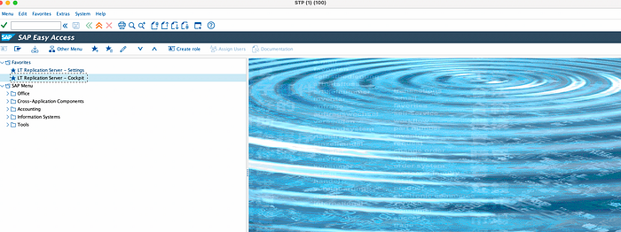
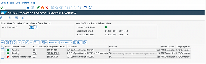
The initial screen of the SLT Cockpit lists all previously created configurations. Each configuration has a unique identifier called Mass Transfer ID (MTID). You can define multiple configurations in a single SLT. Each configuration is a combination of the source and target system with specific replication settings. Within this environment you can find details to existing SLT data replications and you can also create, monitor and execute additional ones.
Normally, you should have an empty page if it’s your first time configuring the server.
Click the Create Configuration button to define a new one. It opens a wizard that guides you through basic settings. I already did this but I will show how to fill the parameters and skip the creation step.
- Start specifying a user-friendly configuration name and optional description. You don’t have to maintain other fields on this screen.

2. Specify the source system connection, in our case RFC Connection equals none (as we like to load data out of the same system, that also SLT is running on). Click “next”.

3.Specify the target system connection to SAP Data Intelligence. Choose option “Others” and specify “SAP Data Intelligence”.

4. Define the SLT Job Settings. If you plan a simple test of replicating a single table to SAP Data Intelligence, it is fine to provide one job for “Data Transfer Jobs” and as well for “Calculation Jobs”. Otherwise, for production scenario, I recommend setting Number of Data transfer and initial jobs to approximately the number of tables and parallel processes to get them. For the number of calculation jobs, it’s the number of jobs that is run on S/4HANA side, you can set it to a number between 5 and 10 to start and then tune it depending on your SLT infrastructure saturation.

5.Click “next” and then “create”.
6. Note down the Mass Transfer ID, that has been generated. This ID uniquely identifies the SLT Configuration and is required later for the configuration of the SLT Connector operator.
4. Data intelligence pipeline:
Having created the SLT configuration, we are good to start building our pipeline in SAP Data Intelligence.
As explained earlier, Data Intelligence is used to fetch data from SLT queue we will focus on three services: Modeler, Connection Management and Monitoring.
4.1. Build pipeline for SAP table using DI Modeler:
The SAP Data Intelligence Modeler application is based on the Pipeline Engine, which uses a flow-based programming model to run graphs that process your data.
In order to fetch an SAP table data from SLT queue and push it to GCP bucket, we can will use a data intelligence functionality called “replication flows” that performs real-time or batch transfer of data, from source to a target using either full or delta load.

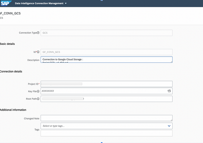
Before building the pipeline, we need to prepare our source (SLT) and target (Google Cloud Storage) connections. To do it, it’s pretty simple using the UI: after logging into the DI cloud launchpad, navigate to Connection Management menu, click on + icon to add a connection and add a first one for SLT (choose ABAP as connection type and fill with SLT configuration parameters):

Same for GCS, add a connection (with GCS type), you need a to specify a GCP Project Id, the name of the GCS bucket and unfortunately a service account key (sorry but we need a key from GCP with Storage editor role on the target bucket).
After preparing the connections, go back into the DI cloud launchpad, navigate to Modeler menu:

Click on the Replications tab located on the left of the navigation pane replication flows :

Click on the + icon on the top to create a replication flow. A pop up would appear to provide a name for the flow, fill a name to your replication flow:
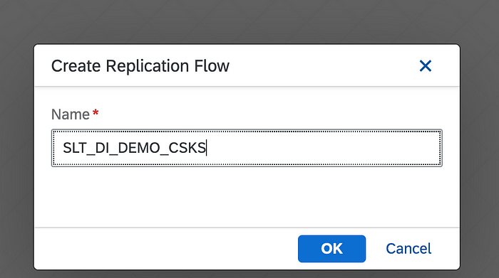
We will see this screen, with 3 tabs: Properties, Tasks and Activity Monitor.
First, where we need to specify source and target configuration in the “Properties tab”:

For the Source Connection choose the SLT system we connected earlier to our DI instance from the drop-down menu. In the corresponding Container section navigate to the SLT folder then select the Mass transfer ID associated with the SLT configuration created previously and click OK.
Following the same process, select the connection for GCS bucket as a target connection and in the corresponding Container section select the folder where the table should be replicated ( just put “/” if you want that the data is pushed in folder with same name as the table) and click on OK button.
After we are done specifying the source and target details, RMS provides additional functionalities like specifying file type in the target (CSV/JSON/Parquet), how we want the Delta records to be grouped in the target (Group by Hour or Date). I decided to choose Parquet ( I would prefer avro but it not available yet) et group by “Date”.
The screen after specifying all the properties should look something like this:

As you constated, we just precised the source and the target parameters, we did not set up yet which table we need to extract …
To do it, switch to the Task tab right next to Properties tab.
We can add more than one task under a single replication flow but let’s keep it simple and have with one task per replication flow (one flow= one table).
Click on the Create button on the top right corner under the Task tab and search for the name of “CSKS” table in the search box and select the table from the list and click OK.

After adding the CSKS table under the Task tab we can also define filters on the table and do some mappings/renaming/filters but for now the focus would be on setting up a simple replication without any mapping or filters.
For the Target, the same name of source table is automatically picked but can be manually changed. In the Load Type we need to specify whether the load would contain both initial and delta or just the initial load. The Truncate functionality can be checked if the user wants to clear up the existing content of the chosen target. In our case, we will choose initial+delta so that we can have an initial full export of the table and then delta load.

Next, save the flow click on the Validate button next to save. Validating the replication flow checks whether the configured replication flow satisfies the minimum requirements. The validation checks are shown in the image below that appears after the validation process completes

Then the next step would be to deploy the replication flow by clicking the Deploy button next to Validate. Deploying the replication flow is a necessary step prior to running it.
After the replication flow is successfully deployed, the Activity Monitor tab would show that deployment has been successful without any errors.

The final step would be to run the flow by clicking the Run button. The current status can be seen in the Activity Monitor.

Additionally, clicking on Go To Monitoring button would open Data Intelligence monitoring application where we can monitor the replication progress and see additional details. Below image shows that the initial load has been completed successfully, and the current status has changed to delta transfer.

You can go now to GCS bucket in GCP environment and check that a new folder “CSKS” appeared with two subfolders, initial and delta:

In the initial folder we will found parquet files corresponding to an inital export of the table:

The delta folder will contains many folders, one per day and each day’s folder contains one or many parquet files regrouping the transactions:

Note: In order to do any changes to the configuration of the replication flow or to reset the entire process the flow needs to be undeployed by clicking on the Undeploy button.
Now, our replication is setup and you will see new files in the bucket whenever new data appeared in SAP system, with just a few minutes of delay.
5. Load SLT data to from GCS to Bigquery:
I hope the first section of the article demonstrated how straightforward it is to replicate an SAP table from an SLT system to a GCS bucket using SAP Data Intelligence Cloud’s RMS functionality in just a few simple steps. Now, let’s move on to an overview of how to push the data to BigQuery. This process is relatively simple, especially if you have experience as a data or cloud engineer, so I won’t go into too much detail.

5.1 Pipeline setup :
In order to ingest data coming from Data Intelligence, in quasi-real time, to Bigquery, we have many possibilities and depends highly on your business refresh needs:
- If you want to keep the real time data ingestion, I recommend setting up an event-based pipeline using EventArc and Cloud run, that listens to the bucket and ingest new data to Bigquery.
- If it’s sufficient to refresh the data a few times a day, we can setup a scheduled pipeline that calls a Cloud run to check if there are new files in the bucket and ingest them. You can also adapt your scheduled pipelines to be executed each hour or even each minutes.
I believe that the two solutions can be easily implemented with different tools. As we are in GCP environment, I suggest to implement a scheduled Cloud Workflows pipeline with 2 steps:
- Move new data from SLT GCS bucket to a landing or a temporary bucket.
- Ingest the data to Bigquery with the required transformation and archive the files to another bucket. I am going to delve into the transformation part because I think it’s the most critical step in the ingestion process and we need to understand what SLT is sending to the bucket and how to reconstruct the SAP table in GCP using the parquet files.
5.2 SLT data transformation in Bigquery:
Below an example on how a parquet file received from Data Intelligence looks like:
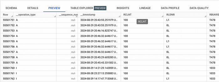
We will have all the table standard columns and additionaly 3 metadata colums:
__operation_type: Identifies the type of the row. The possible values are as follows:
- L: Written as part of the initial load.
- I: After the initial load completed, new source row added.
- U: After the initial load completed, after image of an update to a source row.
- B: After the initial load completed, before image of an update to a source row. These records are only sent by some sources (like SAP HANA) and only when the after image of the update is not passing the filters specified in the replication task.
- X: After the initial load completed, source row deleted. The only target columns to contain data for this operation code are codes that reflect the source key columns. All other target columns are empty.
- M: After the initial load completed, archiving operations
__sequence_number: An integer value that reflects the sequential order of the delta row in relation to other deltas. This column is generally empty (in my experience).
__timestamp: The UTC date and time the system wrote the row
As you saw, we will have many operations in the parquet file and appending the files is not sufficient to replicate the source data, we need to compare the new rows to the actual rows and perform an action depending on the operation type, for example:
- Update: we update the row in the target table (based on timestamp)
- Delete: we delete the row int the target table
- Insert: we append the data
To do so, I suggest performing the following steps in your daily transformation:
- Ingest new data to a staging (temporary) table.
- Apply a merge query between the temporary and the target table based on the operation type, timestamp and the primary keys.
- Delete the temporary table.
Below an example of how we can implement the merge query, you should also apply a deduplication step on the staging table before the merge query.
query = f"""
                MERGE {quote_identifier(str(target_table))} T
                USING
                    (
                    SELECT * EXCEPT (rank) FROM (
                        SELECT DISTINCT *, rank() OVER (
                            PARTITION BY {', '.join(primary_keys)}
                            ORDER BY {timestamp_column} DESC
                        ) AS rank
                        FROM {quote_identifier(str(staging_table))}) stg
                        WHERE stg.rank = 1) as S

                ON {merge_condition}
                WHEN MATCHED AND S.{timestamp_column} < T.{timestamp_column} THEN
                    UPDATE SET T.{timestamp_column} = T.{timestamp_column}

                WHEN MATCHED AND S.{timestamp_column} > T.{timestamp_column} and (S.__operation_type in ('U', 'A', 'I') OR S.__operation_type not in ('X')) THEN -
                    UPDATE SET {update_condition}
                WHEN MATCHED AND S.__operation_type = 'X' THEN
                DELETE
                WHEN NOT MATCHED THEN
                    INSERT {insert_condition}
                """
The query can be optimized by targeting a specific clusters and partitions based on the timestamp columns (useful to reduce query cost for big tables like BSEG or ACDOCA). If you are interested on more details, please ping me on Linkedin and I will share the code and global schema of the architecture already in place.
6. Handle CDS Views:
As explained in the the first section, the process described until now works well when working with SAP tables. Otherwise, we cannot use the standard extraction via SLT for CDS Views because it uses change data capture (CDC) to identify and replicate changes in database tables. Since CDS views do not store data and are simply queries run on top of existing tables, there is no inherent mechanism to capture “changes” in a view. In other words, the concept of tracking updates or inserts that SLT relies on for replication does not apply to CDS views because they are not objects that store data themselve. Moreover, CDS views are often built on top of multiple SAP tables and other views and may involve complex transformations, joins, aggregations, and filtering. Since SLT operates at the table level, it cannot handle these complex logic combinations that exist only in the execution layer of a CDS view.
In my experience, to read a CDS view and write its content to the target system, only SAP Data Intelligence is needed with a direct connection.
To perform the extraction, we need to use “graphs” instead of “replication flows” this time. The process is simple using the UI:

Select “Use Generation 2 Operators” and then you will have an empty graphs and you can add operators:

This flow contains 3 steps: the operator “Read data from S/4HANA” in which we set-up the connection to the CDS view, then the step for “Structured file producer” that generates parquet file with relevant data types and put it into Google Cloud Storage. And the last one “Graph terminator” stops the graph.
For CDS Views, we don’t have the choice, we can only extract them in full mode, so make sure in the “structure file producer step”, make sure to select the “overwrite” as Part File Mode

⚠️ One important detail: we cannot extract CDS views directly unless the tag
@Analytics.dataExtraction.enabledis set to true in the SAP system. Without this setting, the view will not be recognized by SAP Data Intelligence.
Unlike tables, which are extracted using the CDC (Change Data Capture) pattern, graphs need to be scheduled manually; otherwise, the parquet file will not be generated or replaced in Google Cloud Storage.
To schedule the process, you can use the “Run As” or “Schedule” option with Snapshot Configuration enabled.
7. Conclusion:
And that’s it! We’ve covered the main steps for replicating SAP data in a GCP environment. As you saw, the process involves a lot of configuration and manual steps, largely because automating the setup of SLT and creating pipelines isn’t straightforward.
I’ve heard there’s an API for SAP Data Intelligence, though I’m unsure about its current maturity. If it’s reliable, it would likely simplify the process of creating a Terraform provider to automate pipeline creation.
We didn’t go into much detail about monitoring the solution, but it’s crucial since issues can arise with SLT or Data Intelligence due to changes in field types or infrastructure resources. Monitoring the process and preparing for replay scenarios is important. I’ll likely create a dedicated article to show how to export Data Intelligence and SLT logs to BigQuery using ABAP scripts, and how combining this with BigQuery freshness metadata can help monitor pipelines.
I hope this article was helpful! Feel free to share it on LinkedIn, and please let me know if you have any feedback or questions !
To stay updated with my latest posts, you can follow me on Medium! 😃